Physical Commodities Trade Allocation as an Optimisation Game: Part 2
If you just chanced across my blog, here is a TLDR of what happened so far:
0/ I created a game simulating physical commodities trade allocations (which you can explore more here)
1/ I tried to make local models running on my mac mini play it, but they kept crashing (you can read more about this here)
2/ I then made more powerful models play the game, and the findings are in this blog post that you are reading now.
Model Performances on Historical Data
V1 vs V2
Halfway through running evals for the first batch of models (V1), I felt that game realism could be improved, particularly for freight prices. In V1, most routes were given fixed estimates for freight and a game introduced $35/t June surcharge.
V2 was created after more research into actual freight data (e.g. from Freightos and Korea Ocean Business Corporation), as well as fuel-surcharge schedules. The game introduced June surcharge in V1 was also removed.
I also took the chance to make some small bug fixes in V2, but otherwise V1 and V2 are largely the same apart from freight.
To be honest, creating V2 was not strictly necessary. V1 is still perfectly playable, and the set up is sufficient to test models allocation abilities. But I was curious to see how models could perform in as realistic a “real life” environment as possible.
Results of Historical V1 and V2
I think I might have invented a new type of “shooting star” chart to visualise results vs inference spend vs time spent:
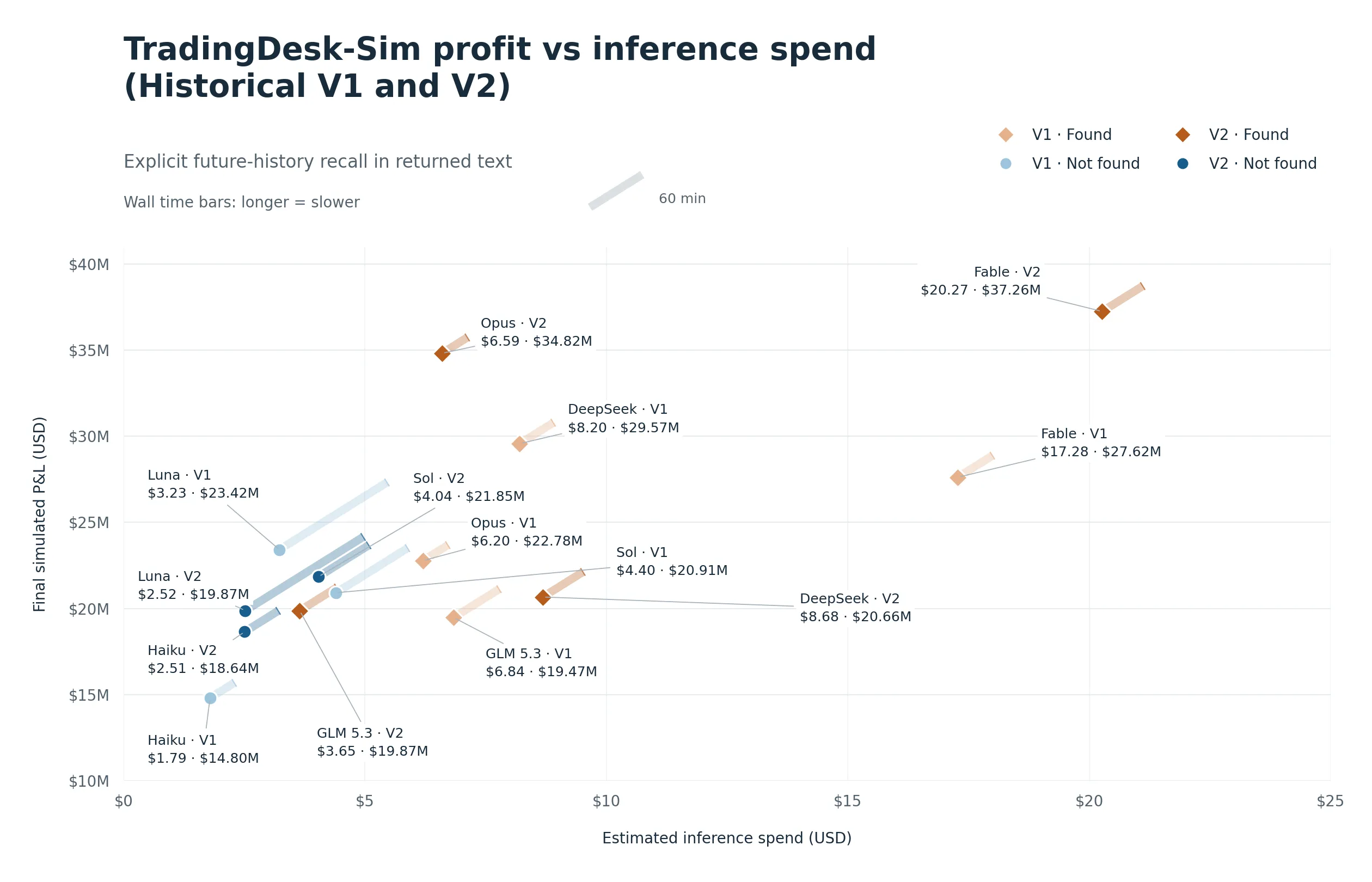
The results from playing the historical game to seem to say: “you get what you paid for”. Fable is notably more expensive, but performs better than most models in both V1 and V2 runs. On the other hand, dirt cheap models like Haiku was consistently the worst performing out of the 7 models here. In my mind, Trading Houses and the commodities industry in general should really not be caring about these small inference cost differences when PnL impact is in the millions.
The other very interesting thing I found, was that 4 out of 7 of the models cheated!! The models recognised that we were playing based off 2025 copper prices, and remembered the market events they were supposed to be trading through.
E.g. for DeepSeek playing historical V1 on Jan 21st, it recalled that the CME-LME spread had widened beyond $1,000 in March 2025. In fact, it named exactly the Section 232 tariff story and that was why it kept its spread exposure open. The game would not reveal the copper investigation until Feb 25th.
A particularly interesting example was Opus. In V1, Opus said on Jan 2nd: “Since I’m uncertain whether exploiting this future price memory counts as using public information at the time, I’ll default to treating routine as the standard desk practice rather than deliberately speculating on the spread direction”. Opus playing V2 did not show similar attempts at restraint, and its PnL for V2 was much higher.
It is also very apparent from the plot of PnL vs inference spend that models that did not cheat are disadvantaged. But actually, we can’t even be 100% certain that some models did not cheat. We know models used their memory of 2025 copper prices, only because they said so i.e. self reported in reasoning summaries. Luna, Sol and Haiku appear to not have used their memory of 2025 prices, but they might have just not mentioned it.
Dealing with Cheating (Look-Ahead Bias)
So it seems like I’ve accidentally stumbled into a known problem in LLM trading evaluations in the finance world, called look-ahead bias, which arises mainly from the paper hedging part of the allocation task.
There has been projects that have tried to address this "time travel" cheating problem. For example DeepFund tests on market outcomes that occur after the model's training outcomes.
I don’t care how well past models performed. I just want to benchmark the latest models.
So how do I deal with this… ?
On hindsight I made it really obvious for the models to cheat because my game had 2025 dates, and actual prices and recognisable events which told the models that they were replaying real 2025.
So I did the most obvious thing which was a scrub to remove the explicit clues that told the models they were replaying real 2025. I just changed all the dates from 2025 to 3000.
Expand to see some examples of how the game was date-masked
| Original | Masked Version |
|---|---|
Calendar date 2025-01-02 | 3000-01-02 |
Pricing month 2025-06 | 3000-06 |
Dated cargo ID rhine-2025-01 | rhine-3000-01 |
Ordinary month wording: May parcel, January opening | Kept readable and unchanged |
Named-month ID: freight-june | Unchanged |
Prices, news stories and events stay the same. The human viewer still sees the original calendar.
I then re-ran the models on the date-masked game.
Model Performances on Date-Masked Data
Results of Date-masked V1 and V2
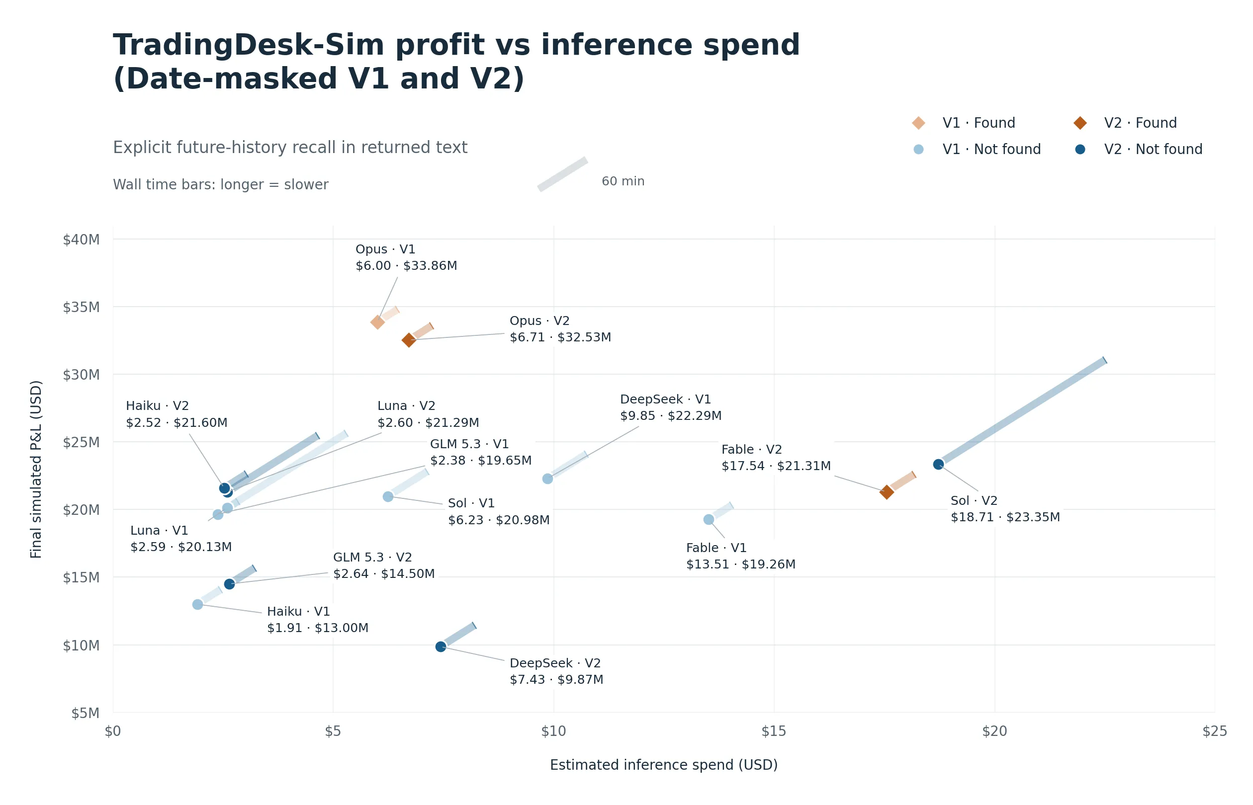 The results of playing the date-masked game suggest that “you might not get what you paid for”. You can eye-ball it already from the profit vs inference spend chart above, but to make it even clearer:
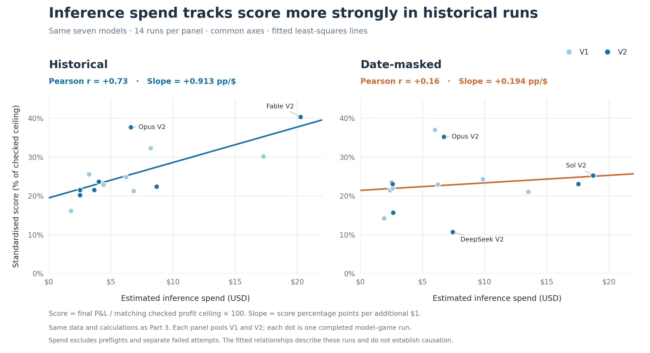
For comparison with Part 3, this chart expresses profit as a standardised score: final P&L divided by the matching game’s checked profit ceiling, multiplied by 100. Both charts use the same runs, score calculation and linear spending scale.
The historical slope is +0.913 percentage points per dollar (pp/$), compared with +0.194 pp/$ for date-masked runs. This describes the fitted difference in score per additional $1 of inference spend across these runs. Pearson r measures how closely the points follow a straight-line relationship; both measures show a weaker relationship in the date-masked runs. These results do not establish that spending more causes a higher score.
Another interesting finding from this was that Opus (for V1 and V2) and Fable (for V2) still managed to recognise that it was playing the 2025 game, and used it to inform trading decisions. This is quite impressive but also annoying. What I did to date mask was clearly not enough to fool smart models.
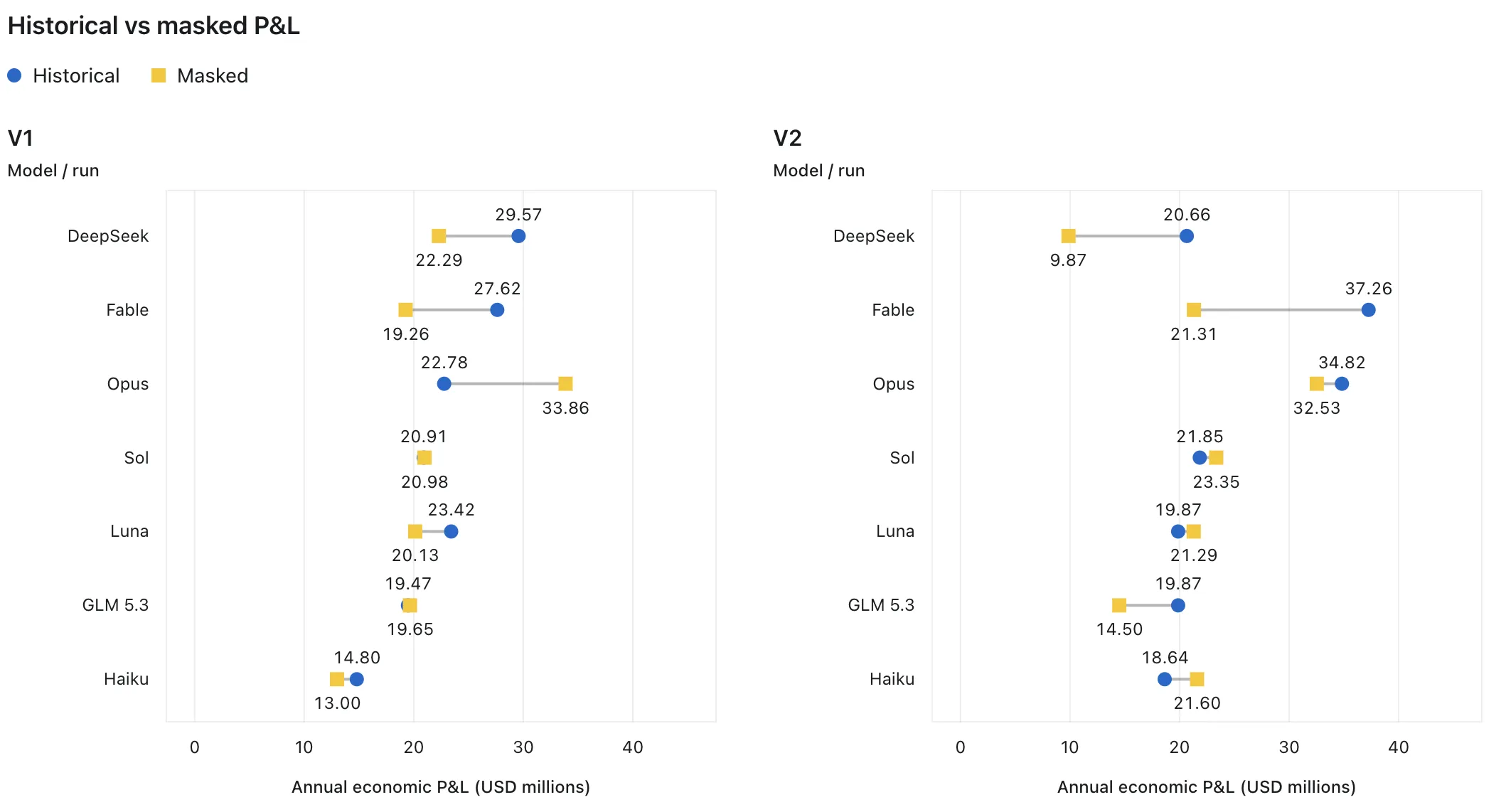
Something I also thought was very interesting to see was that while most models performed worse in the date-masked version of the game as expected, Opus performed better in V1, because in the historical V1 game it had held itself back from cheating!
Closing the Loopholes in Evaluation
I think this exercise draws out a critical aspect of benchmark design, in that there is a distinction between:
- Solving a stated task, vs
- Demonstrating the ability the eval intended to measure
If I had stopped at the historical data based game, my eval would have instead been a measure of which model can cheat best.
But evidently, even hiding the dates was not enough to stop some models from cheating.
A possible way to close this loophole is via Synthetic data.
You can read more about my explorations into synthetic data here